
More and more frequently, we hear about semantic search and new ways to implement it. In the latest version of OpenSearch (2.11), semantic search through sparse vectors has been introduced. But what does sparse vector mean? How does it differ from dense matrix? Let's try to clarify within this article.

If you’re familiar with conventional search engines and technologies like opensearch and elasticsearch, you’ve likely come across tf-idf and bm-25—two algorithms leveraging sparse structures for document representation and relevance calculation. To simplify the explanation of sparse structures, let’s consider a database with three documents:
Representing these documents in an incidence matrix:
| quick | brown | fox | jumps | lazy | dog | sleeps | the | and | a | |
|---|---|---|---|---|---|---|---|---|---|---|
| Document 1 | 1 | 1 | 1 | 1 | 0 | 0 | 0 | 1 | 0 | 0 |
| Document 2 | 0 | 0 | 0 | 0 | 1 | 1 | 1 | 1 | 0 | 1 |
| Document 3 | 0 | 1 | 1 | 0 | 1 | 1 | 0 | 2 | 1 | 0 |
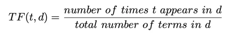
Utilizing the same matrix, we can compute the frequency matrix using the formula:
| quick | brown | fox | jumps | lazy | dog | sleeps | the | and | a | |
|---|---|---|---|---|---|---|---|---|---|---|
| Document 1 | 0.25 | 0.25 | 0.25 | 0.25 | 0 | 0 | 0 | 0.25 | 0 | 0 |
| Document 2 | 0 | 0 | 0 | 0 | 0.33 | 0.33 | 0.33 | 0.33 | 0 | 0.33 |
| Document 3 | 0 | 0.33 | 0.33 | 0 | 0.33 | 0.33 | 0 | 0.67 | 0.33 | 0 |
Finally, applying the formula:
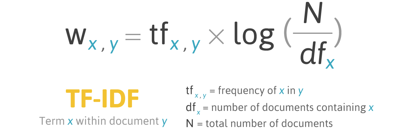
We can visualize the matrix employed in a tf-idf algorithm, which is used to calculate relevance:
| quick | brown | fox | jumps | lazy | dog | sleeps | the | and | a | |
|---|---|---|---|---|---|---|---|---|---|---|
| Document 1 | 0.044 | 0.044 | 0.044 | 0.146 | 0 | 0 | 0 | 0 | 0 | 0 |
| Document 2 | 0 | 0 | 0 | 0 | 0.058 | 0.058 | 0.195 | 0 | 0 | 0.058 |
| Document 3 | 0 | 0.058 | 0.058 | 0 | 0.058 | 0.058 | 0 | 0 | 0.058 | 0 |
You may have noticed, as illustrated in the matrix above, that the values are predominantly concentrated around a few non-zero entries, while the majority remain at zero. This concentration of non-zero values amidst a sea of zeros characterizes what is referred to as “sparse vectors”.
The sparsity in these vectors allows for more efficient storage and computation: it reduce redundancy, as only the non-zero elements need to be stored, leading to more compact data structures. This efficiency is particularly beneficial when working with large datasets, as it enables faster computations and reduces memory requirements.
Using sparse vectors, we have essentially represented the essence of each document by employing a set of numerical values, with a significant portion of them being 0s.
Dense vectors will allow us to do the same, without relying on 0s. In dense vectors, every document is represented by a vector where each values is included between 0 and 1. Each value will represent a feature of our document.
Let’s try to deep dive into how dense vectors work using an example. We have some documents, each of them representing a different animal. To describe every animal we will use some common features. For example, the size, the friendliness and the intelligence.
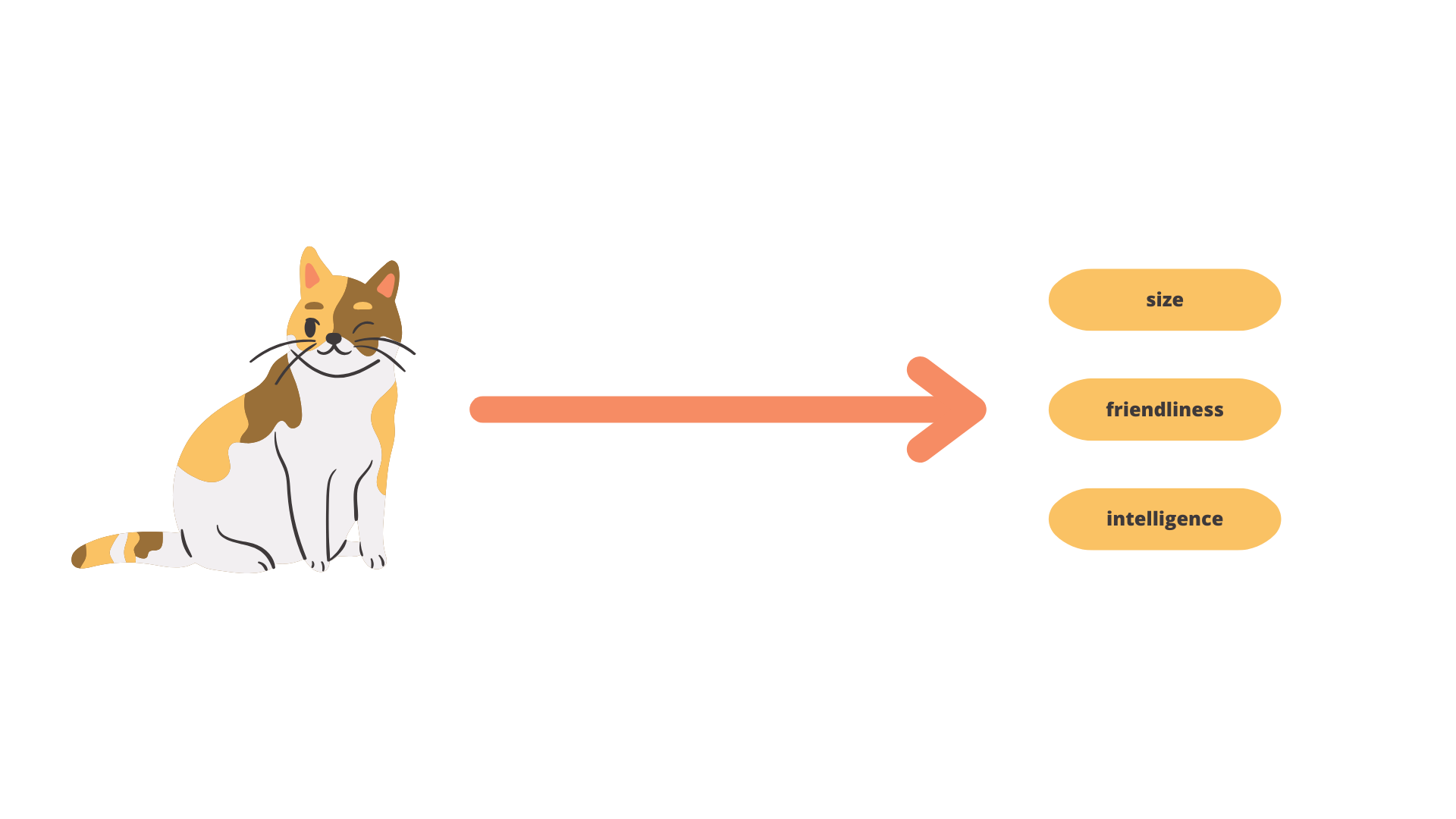
For each feature we can assign a value from 0 to 1, where 0 means less and 1 more. For example, a cat is a quite friendly animal, small size and extremely clever (despite it likes to sleep all the time).
So we can transform our cat and all the animals of our collection into vectors:
| Animal | Size | Friendliness | Intelligence |
|---|---|---|---|
| Cat | 0.25 | 0.85 | 0.80 |
| Dog | 0.30 | 0.90 | 0.80 |
| Elephant | 0.90 | 0.70 | 0.60 |
| Dolphin | 0.60 | 0.95 | 0.85 |
| Parrot | 0.15 | 0.80 | 0.75 |
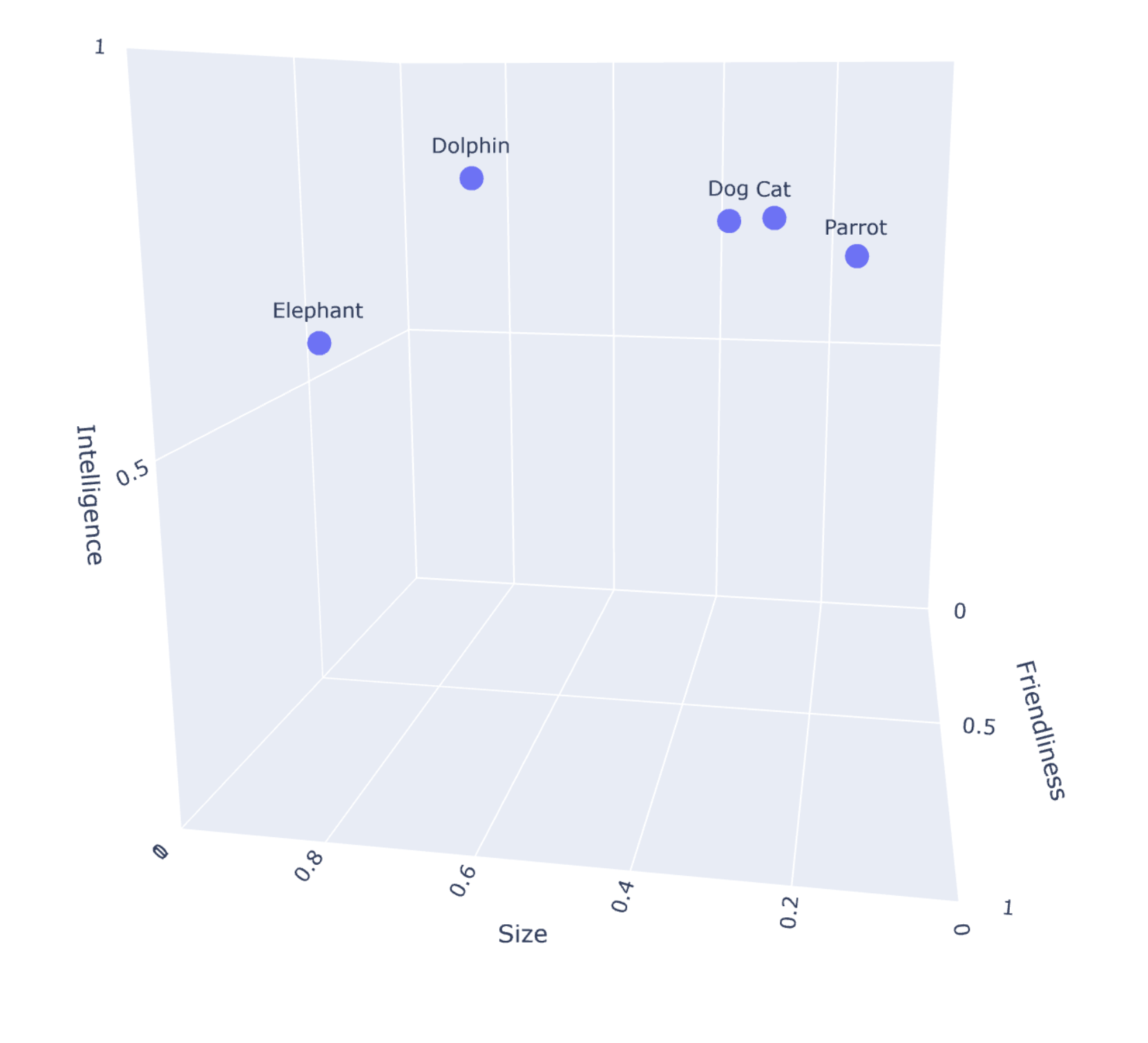
As you may have noticed, we represented the collection using vectors without adopting 0 values. Additionally, each document is characterized by specific features, enabling easy comparisons. Indeed, we can easily represent this 3-dimensional vectorial space using a 3d-graph.
The process of creating dense vectors is typically accomplished using specific models. These models generate vectors of several dimensions, often in the hundreds. While the animal example was relatively straightforward with a three-dimensional vector, envision dealing with a 784-dimensional vector. This complexity suggests that generating these vectors can indeed be time-consuming and require more space than what we typically encounter with sparse vectors.
In vector or semantic search, we are essentially comparing our vectorial database to a query vector. The query vector is essentially our query transformed into a vector.
The comparison between the query vector and the database can be made through different mathematical functions, such as the cosine similarity or the dot product distance. The most similar documents to our query vector are the most relevant documents, and, normally, the documents we are looking for.
If you want to learn more about how vector search works, and how to implement it, you may want to give a look to Exploring Vector Search with JINA. An Overview and Guide and Diving into NLP with the Elastic Stack.
Semantic search can be done also through sparse vectors, thanks to a technique called “Term expansion”.Term expansion involves broadening the representation of a document by incorporating additional relevant terms that may capture the meaning of the document. These expanded terms are indexed as if they were initially part of the document,. In this context, machine learning models, such as Elasticsearch’s “elser” or Amazon’s Neural Encoder for OpenSearch, can be employed for effective term expansion.
Let’s see how this works, once again, through examples:
As we did before, let’s consider this phrases
and their incidence matrix:
| quick | brown | fox | jumps | lazy | dog | sleeps | the | and | a | |
|---|---|---|---|---|---|---|---|---|---|---|
| Document 1 | 1 | 1 | 1 | 1 | 0 | 0 | 0 | 1 | 0 | 0 |
| Document 2 | 0 | 0 | 0 | 0 | 1 | 1 | 1 | 1 | 0 | 1 |
| Document 3 | 0 | 1 | 1 | 0 | 1 | 1 | 0 | 2 | 1 | 0 |
Term expansion aim to associate new relevants words to each documents. For example the term quick can be expanded using different synonymous, such as fast or swift. This can be done for each term and for each phrase in our database.
For example:
which will result into a new incidence matrix
| quick | fast | swift | brown | fox | animal | jumps | lazy | dog | sleeps | the | and | a | … | |
|---|---|---|---|---|---|---|---|---|---|---|---|---|---|---|
| Document 1 | 1 | 1 | 1 | 1 | 1 | 1 | 1 | 0 | 0 | 0 | 1 | 0 | 0 | — |
| Document 2 | 0 | 0 | 0 | 0 | 0 | 1 | 0 | 1 | 1 | 1 | 1 | 0 | 1 | — |
| Document 3 | 0 | 0 | 0 | 1 | 1 | 1 | 0 | 1 | 1 | 0 | 2 | 1 | 0 | — |
Now, if we search for ‘naps,’ we will retrieve the second document where ‘A lazy dog sleeps.’
Similar to semantic dense vector search, sparse semantic search can also employ the machine learning model during the search phase to expand our query. In this case, we are referring to bi-encoders in dense vector search. If we use term expansion only during indexation, we are in ‘document-only’ mode. This second solution is much faster since there is no term expansion at runtime.
Sparse search has three big advantages compared to dense vector search:
In this exploration of sparse and dense vectors, we delved into the foundational aspects of search engines. We covered the traditional use of sparse vectors in algorithms like tf-idf and bm-25, as well as more modern techniques involving both dense and sparse vectors for semantic search.
It’s crucial to remember that the choice between keyword search and semantic search depends on the specific requirements of a given application, and vector search may not always be the most efficient solution. Furthermore, deciding between sparse and dense vectors can be challenging and requires a thorough requirements analysis.
In conclusion, the landscape of information retrieval continues to evolve. Understanding the strengths of both sparse and dense vector approaches is essential for building effective and scalable search systems and we hope this article helped to clarify every difference.